DNA-PAINT and Super-Resolution Microscopy

Breaking light’s diffraction limit, spectrally unlimited multiplexing, and probing single-molecule events with DNA-PAINT

You probably already know a bit about super-resolution microscopy and many acronyms that denote the flavors it comes in, like STEM, PALM, STORM, STED, SIM… It’s an incredible array of techniques that essentially uses some clever physics and chemistry to overcome a microscope’s resolution limit, which is based on the diffraction of light, and so lets you look at very small things that are very close together. But have you heard of super-resolution microscopy and DNA-PAINT?

Before we get into DNA-PAINT, let’s start with a little bit of background about where this technique came from. 

PAINT: labeling without labeling

Points accumulation for imaging in nanoscale topography (PAINT) came about in 2006 (Sharonov & Hochstrasser, 2006) as a very interesting way to image biological structures beyond the diffraction limit – down to 25 nm in this case. (Keep in mind that your regular light microscope has a resolution limit of around 200 nm due to the diffraction of light.) 

Rather than labeling individual target molecules with fixed fluorophores like in other super-resolution techniques, PAINT relies on continuous and freely diffusing fluorescent probes in solution. These probes wash over and collide with the target, which generates a fluorescent “spike”, or signal, in the form of a diffraction-limited spot on whatever object the probes become collide with and get stuck on. 

The authors explain how “Each probe that hits the object and becomes immobilized is located with high precision by replacing its point-spread function (PSF) by a point at its centroid.” PAINT lets users image the outline of structures like phospholipid bilayers and even vesicles at nanoscale resolution without the need for direct labeling.

What is DNA-PAINT?

While PAINT overcomes some of those pesky super-resolution microscopy issues to do with dye photophysics, it’s still somewhat limited as it relies on the fluorescent solution having things like hydrophobic interactions or electrostatic coupling with the target. But with the advent of DNA nanotechnology, it became possible to combine the benefits of PAINT with a more controllable target–probe interaction that uses DNA molecules as both imaging and labeling probes, or ‘strands’.

In DNA-PAINT, strands come in two types:

• Imager strands: single-stranded short oligonucleotides conjugated to an organic dye that diffuse freely in the imaging buffer and which bind to docking strands
• Docking strands: complementary oligonucleotides bound to the target you’re interested in (bound via standard immunolabeling using DNA-conjugated antibodies or even by hybridizing docking strands to DNA or RNA molecules) 

Unbound, the camera doesn’t detect imager strands as they diffuse over multiple pixels per frame. But once the imager strand binds its complementary docking strand, fixing it in one place for a while, the camera accumulates enough photons from the dye to be detected. Together, bound in a DNA duplex, these strands create the classic fluorophore ‘blinking’ you need for stochastic super-resolution microscopy. 

And since the stability of this DNA duplex is the exclusive determinant of how long strands remain in a bound state, the user is given a great deal of control over the subsequent blinking kinetics. For example, you could change the time in a bound state by adjusting strand length, guanine-cytosine content, temperature, or imaging buffer composition. It’s worth remembering that your control over blinking kinetics is independent of dye properties, giving you the freedom to use almost any single-molecule-compatible dye. 

The final result is a type of single-molecule localization microscopy (SMLM) that can give you resolution down in the 5–10 nm range and allows multiplexing with a single laser source. Clearly, DNA-PAINT has fantastic potential within the realms of biological imaging (when what you need to image is very, very small!).

In a wonderfully detailed protocol on how to use DNA-PAINT and super-resolution microscopy (Schnitzbauer et al., 2017), the authors show how to get novices and expert users using not only DNA-PAINT but also ExchangePAINT (a multiplexing option limited only by the number of orthogonal DNA sequences) and qPAINT (which allows for quantitative imaging) without the need to already be familiar with super-resolution microscopy. We highly recommend you give this paper a read.

Using DNA-PAINT to look at synaptic stabilization and elimination

So how are researchers using DNA-PAINT? Well, one group wanted to see how, during brain development, synapses are chosen for stabilization or elimination after formation (Gomez-Castro et al., 2021). When postsynaptic adenosine receptors are muted or do not find enough extracellular adenosine, synapses get eliminated.

It was already known that GABA and GABA type A (GABA_A) receptors (GABA_ARs) play a role in this synaptic stabilization vs pruning, and that adenosine A_2A receptors (A_2ARs) can detect the corelease of adenosine triphosphate (ATP) and adenosine with GABA. So, Gomez et al. looked specifically at adenosine signaling in GABAergic synapse stabilization and elimination. 

Using mouse hippocampus samples, Gomez et al. used electron microscopy to show postsynaptic localization of A_2ARs with what they presumed to be GABAergic synapses. To confirm this result, they used DNA-PAINT with our Anti-Adenosine A2A Receptor Antibody (#AAR-002) to clearly show that A_2ARs were indeed positioned close to GABAergic post-synapse, (which they identified by the presence of gephyrin – a scaffolding molecule). These data, along with western blot and quantification of DNA-PAINT, revealed an increased density of postsynaptic A_2ARs during the peak of synaptogenesis.

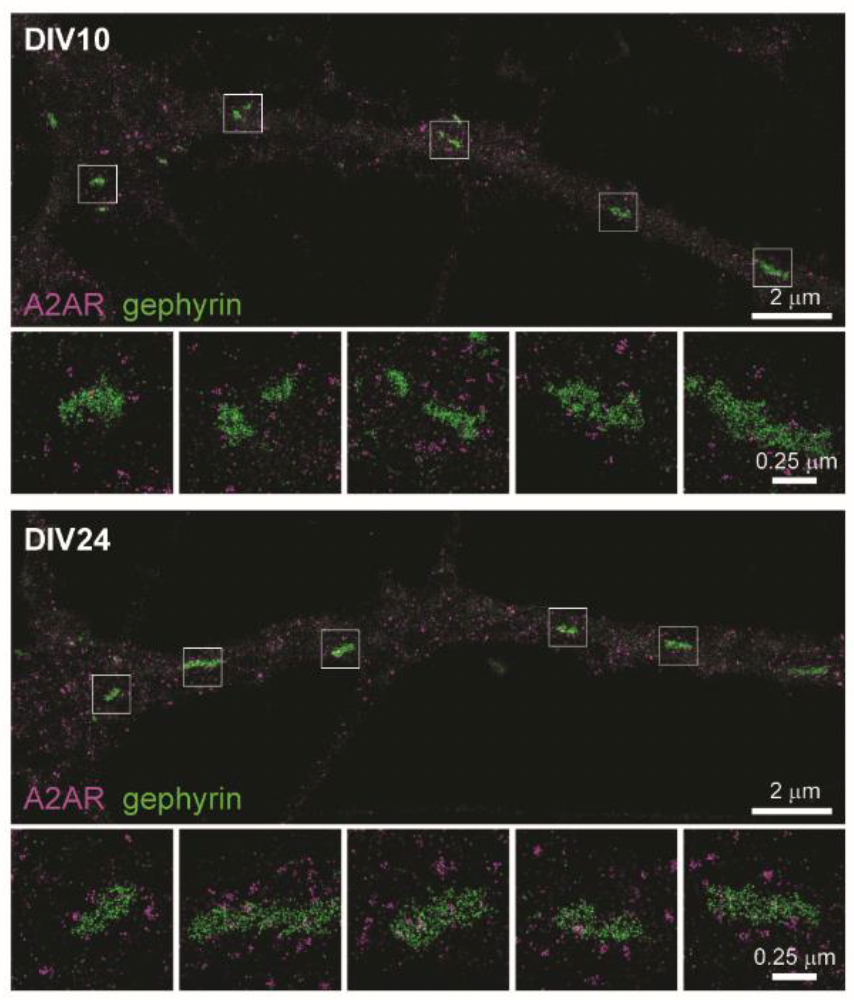
Their work showed that through an autonomous mechanism, A_2ARs stand ready to detect active GABAergic synapses that release GABA and ATP/adenosine, which push a synapse’s fate towards stabilization or elimination after those synapses become inactive. 

Using DNA-PAINT to look at GPCR oligomerization

Technically the paper we’re about to mention uses qPAINT, the quantitative version of DNA-PAINT, but the principle is the same. Just quickly, you remember how DNA-PAINT relies on imaging and docking strands? Well, qPAINT relies on how the frequency at which imager strands bind to their docking strand scales linearly with the number of docking strands, and, coupled with the predictable blinking kinetic, qPAINT lets you undertake quantitative analyses. 

This work from Joseph et al. (2021) wanted to show the power of qPAINT by looking at the nanoscale distribution of the P2Y₂ receptor, a rhodopsin-like G-protein coupled receptor (GPCR), in a pancreatic cancer cell line. The reasoning behind this was that while we know GPCRs form dimers and oligomers, and that oligomers can behave differently from monomers (in areas like pharmacology and function) (Guo, et al., 2021), traditional imaging techniques haven’t provided good data on the size of these oligomeric complexes or GPCR location in the cell. Admittedly, some imaging work has given average oligomerization information, but they still lack precise stoichiometry of specific molecular complexes. 

Hence, DNA-PAINT, well, qPAINT. The researchers chose P2Y₂ as it’s been tied to a whole variety of physiological processes, like immunity and bone mineralization, but also several cancers, including breast, prostate, and pancreatic.

In fixed ASPC-1 cells (a line from pancreatic ductal adenocarcinoma), the researchers used our Anti-P2Y2 Receptor Antibody (#APR-010), which binds to the third intracellular loop between the fifth and sixth transmembrane domain of P2Y₂, for immunofluorescence and the DNA-antibody-coupling reaction (where the antibody is chemically coupled to an optimized docking strand sequence). They used DNA-PAINT to prove where the receptors were and qPAINT to get an idea of the quantities (Figure 2). 

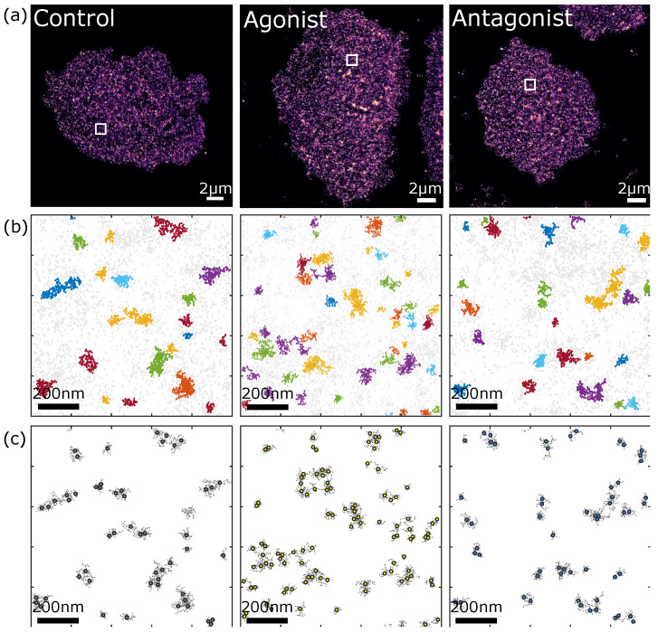
So, what did the imaging and data analyses show? Firstly, being able to visualize individual receptors, the work has offered up an invaluable quantitative characterization of the P2Y₂ receptors’ density, spatial organization, and stoichiometry in AsPC-1 cells. But, if you want to be specific, they found that 

• P2Y₂ receptors are highly expressed in AsPC-1 cells with an average density of around 40 receptors per μm²
• P2Y₂ receptors exist mainly in nanodomains composed of three or more sub-units
• Only 20% of the P2Y₂ receptors exist as dimers while 10% exist as monomers
• The agonist (ATP) didn’t affect P2Y₂ receptor oligomerization status, but the antagonist (AR-C 118925XX) did reduce the percentage of P2Y₂ receptors that form oligomers
• Homo-oligomeric assemblies of P2Y₂ receptors are likely needed for receptor internalization 
• P2Y₂ receptor oligomeric assemblies might just be part of the receptor’s natural activation

Some really interesting stuff – and visualizing individual receptors will always be a fascinating concept!

Super-resolution for the cell biologist

So, we’ve established that super-resolution microscopy and tools like DNA-PAINT are wonderful for looking at the incredibly small. But in biology, we want to look at the incredibly small, sure, but we want to do it when those incredibly small things are in motion. Whether it’s cytoskeletal dynamics or axonal transport, so much of what we study is moving somewhere. So, can super-resolution help with live-cell imaging?

In short, yes. And when it comes to super-resolution live-cell imaging, with fluorescence, the primary goal is the keep the sample alive! Avoiding the build of phototoxicity is what will make or break a super-resolution method.

Without getting into the details (we’ll save that for another blog!) here are some examples of super-resolution techniques that work in live cells. 

Fluctuation-based super-resolution microscopy

This uses algorithms to analyze the oscillating changes of a fluorophore’s state (essentially ‘on’ and ‘off’) to build up a picture of where those fluorophores are at an enhanced resolution.

Pixel reassignment super-resolution microscopy

Here, the usual photomultiplier tube is swapped out for an array detector, that takes each detected element and reassigns it in space to achieve a smaller PSF, giving you a higher resolution. 

Structured illumination microscopy (SIM)

With this method, your sample is illuminated with patterned light – achieved by placing a fine grating in an intermediate focal layer or by using a spatial light modulator (SLM). Images are taken in different focal planes using a different pattern, which an algorithm combines into a super-resolved image. There’s a lot more detail in here about shifting images between different frequencies, and if you’d like to read more about the specifics, take a look at a paper by the physicist, Susan Cox (2015). SIM is commonly used for live-cell imaging, but a variant known as SIM-TIRF is usually a better option. 

If you’re interested in pursuing live-cell imaging, whether for super-resolution or not, you should consider extracellular antibodies. These are antibodies that we have designed to specifically target the extracellular portion of a protein – meaning you don’t need to fix and permeabilize cells to achieve antibody-binding.

Photo by Erik Mclean