Imaging mass cytometry and when biology stops being linear
If you’ve worked with antibodies long enough, you know the drill: find your target, get your signal, count your cells, write up your figure legend. Nice, neat, and flat – just like the tissue on your slide.
But the rise of spatial proteomics, particularly techniques like imaging mass cytometry (IMC), is challenging that whole approach. Biology, it turns out, is anything but flat. Beyond which proteins a cell expresses, the real insight is where that cell sits, who it talks to, and what else is going on in the neighborhood.
The Importance of Location, Location, Location
Spatial proteomics changes the questions you can ask by making location an explicit variable rather than a background detail. Instead of “is p75 expressed in this tumor?”, spatial proteomics asks:
- Which cells express p75?
- Are they near nerves?
- Are they clustered with other stromal subtypes?
- Does expression vary at the invasive edge vs the core?
- Is it enriched in hypoxic zones, fibrotic zones, or inflammatory zones?
In a study of over 1,000 non-small cell lung cancer (NSCLC) patients (1), researchers used IMC to map cancer-associated fibroblast (CAF) phenotypes in an impressive amount of detail, taking into account 45 markers. CAF phenotypes were defined using marker expression interpreted within spatial context. The ‘good’ CAFs – like inflammatory CAFs and interferon-response CAFs – turned up in immune-infiltrated, inflamed zones. The ‘bad’ CAFs – including matrix-remodeling and tumor-like CAFs – were found deeper in the tumor mass, excluding immune cells and correlating with relapse.
So Where Does p75 Come in?
Our Anti-p75 NGF Receptor (extracellular) Antibody (#ANT-007) was used in one of the landmark IMC studies on CAF heterogeneity in breast cancer (2). In the tumor microenvironment, p75 serves as a marker of niche fibroblast populations with developmental or stress-associated profiles. But its expression isn’t random. With spatial proteomics, we see that p75 positive cells tend to cluster in specific microenvironments – often at tumor–stroma interfaces, or near neural or vascular structures.
As a result, p75 signal contributes quantitative, spatial, and contextual information rather than a simple presence-absence readout. It contributes to identifying cell phenotypes and deciphering spatial organization.
Antibodies That Perform Under Pressure
Not all antibodies are built for this. IMC uses harsh antigen retrieval, metal conjugation, and ultra-dense multiplexing. Background becomes a bigger problem. So does non-specific binding. A poorly performing antibody doesn’t just muddy one channel – it can compromise interpretation of dozens.
That’s why performance in traditional immunohistochemistry (IHC) or western blot isn’t enough. You need antibodies that:
- Recognize the target epitope in formalin-fixed, paraffin-embedded (FFPE) tissue
- Tolerate antigen retrieval
- Don’t cross-react with common off-target proteins in stromal or immune populations
- Show consistent spatial patterns that match known biology
Alomone’s anti-p75 antibody passed those tests. It was included in a highly selective IMC panel and helped identify fibroblast subtypes that would otherwise go undetected. This nearly demonstrates that the antibody contributes interpretable signal in spatially resolved, proteomic-scale experiments.
When Spatial Resolution Outpaces Antibody Thinking
The same constraint shows up outside IMC. In a recent Nature study introducing Pathology-oriented multiplexing (PathoPlex), researchers showed that integrating biological layers – cell identity, subcellular localization, and signaling activity – breaks down when antibody panels are poorly composed or insufficiently controlled (3). By iteratively imaging more than 140 commercial antibodies at subcellular resolution across archival FFPE tissues, the study demonstrated that spatial protein patterns (“clusters”) capture disease features invisible to single-marker or cell-centric analyses.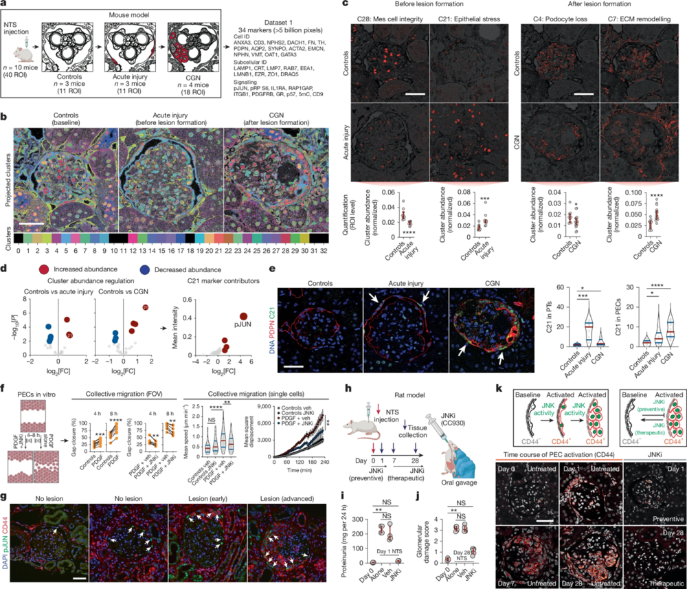
Figure 1. Identification of epithelial JUN activity as a key switch in immune-mediated kidney disease. a, Schematic overview for the proof-of-concept experiment in a mouse model of immune-mediated kidney disease before (acute injury) and after (CGN) pathological lesion formation (n = 10 mice; ROIs = 40). NTS, nephrotoxic serum; details of the antibody panel are provided in Supplementary Table 1. b, Spatiotemporal distribution of colour-coded clusters. c, Examples of interpretable clusters (C28, C21, C4 and C7) of biological significance. Each dot represents an ROI, which was used as an independent observation (n = 11 ROIs for controls, n = 11 ROIs for acute injury and n = 18 ROIs for CGN) and red bars represent medians and inter-quartile ranges. Mes, mesangial. d, Identification of C21 (with pJUN as a top contributor) as a key regulated pathomechanism before and after lesion formation. e, Images of the spatiotemporal distribution of C21 (left) and cell-specific frequency (right) among tubular epithelial cells and PECs. f, Treatment with a JNK inhibitor (JNKi) reduces the PDGF-mediated collective migration of murine PECs in vitro. In ‘collective migration’, error bars represent upper and lower limits. Data are from four biological replicates. Veh, vehicle. g, Confirmation of pJUN expression in PECs during different lesion stages among human kidney biopsy samples (n = 12 patients and n = 3 healthy individuals), which was also associated with CD44 co-expression. h, Schematic overview of the use of a JNKi as a preventive strategy (before NTS) and a therapeutic strategy (7 days after NTS) during the progression of immune-mediated kidney disease in a rat model of CGN. i,j, Proteinuria (n = 4 rats for all groups) and glomerular damage (n = 4 rats for day 0, n = 6 rats for all other groups; red bars represent medians and interquartile ranges) show a direct preventive (i) and therapeutic (j) effect of the JNKi. k, Using expression of CD44 as a readout of PEC activation, we confirmed the effect of the JNKi on PEC activation (using all rats available from i and j). Differential cluster abundance analysis used a two-sided t-test. Cluster composition analysis relied on a two-sided t-test with Holm–Šidák correction. For other comparisons, two-sided Mann–Whitney, Kruskal–Wallis with Dunn, analysis of variance (ANOVA) with Dunnett T3 or ANOVA with Holm–Šidák tests were used depending on the number of comparisons. ****P < 0.0001, ***P < 0.001, **P < 0.01, *P < 0.05 or not significant (NS). Scale bars, 50 µm (c,e,g,k). Diagrams in a, f and h were created using BioRender (https://biorender.com). Image adapted from Kuhel et al. (2025), https://doi.org/10.1038/s41586-025-09225-2 Licensed under Creative Commons Attribution 4.0 International (CC BY 4.0).
In that framework, antibodies functioned as spatial constraints as much as molecular probes. For example, Anti-Aquaporin 2 Antibody (#AQP-002) was used to resolve collecting duct architecture and tubular stress states, where correct membrane localization was essential for cluster interpretation (Figure 1). Without antibodies that preserve specificity and spatial fidelity across dozens of iterative cycles, those higher-order patterns would be missed.
The patterns seen here, reflect changes in protein expression, subcellular localization, and neighborhood context, meaning antibody performance directly determines what biology could be resolved at all.
Spatial Biology isn’t Going Away
As the CAF and PathoPlex studies make clear, the next generation of biomarker discovery probably isn’t going to come from single-marker IHC. Instead, it’s going to come from spatial profiling – of tumors, immune infiltrates, and stromal niches. And that means researchers will need antibodies they can trust in complex, high-plex, spatial contexts.
If you’re building an IMC panel, developing spatial omics workflows, or just trying to make sense of cell identity in messy tissue environments, don’t treat antibody selection as an afterthought. The right reagent allows for spatial interpretation by preserving signal specificity across complex tissue contexts.
 Antibody")
